The Test Mountain Bike: Transition Covert C
My Question/s
- Does tire air pressure affect the rolling resistance of a mountain bike?
- Is the effect the same on both smooth and rough surfaces?
My Hypothesis:
- If the air pressure is decreased by 10 psi, then the elapsed time in which the bike rolls down the track will increase by ~3% because the rolling resistance of a bicycle tire is inversely related to the air pressure.
Variables
Independent Variable (IV)- Also called manipulated/explanatory variable or predictor.
| Independent Variable | How will you Change the independent variable |
|---|---|
| Air Pressure | Decrease the air pressure 10 PSI (Pounds Per Square Inch) at a time |
Dependent Variable (DV) - Also called the response/target variable
| Dependent Variable | How and when will you measure the dependent variable |
|---|---|
| Time in secs | With an iphone stopwatch/When the bike crosses the fixed marker (set at 20 meters) |
Control variable: Variables that are kept the same.
| Control Variable | How will you will control it |
|---|---|
| Rider | Same rider (Mark Kenner) |
| Bike | Same bike (Transition Covert C) |
| Distance the bike rolls | 20 meters |
| Same Tires | Maxxis EXO DHF front and DHR rear, 26” diameter and tubeless |
Materials and Procedures
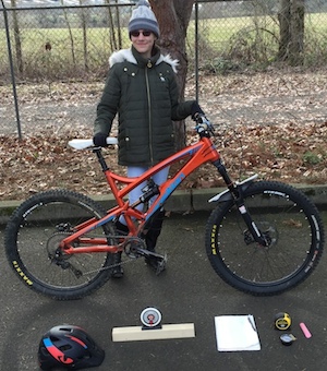
Materials
- Rider (Mark Kenner)
- Assistant/Timekeeper/Statistician/Data-Scientist (Tara Kenner)
- Bicycle (Transition Covert C)
- Tires (Maxxis EXO DHF front and EXO DHR rear, 26” diameter and tubeless).
- Elapsed time will be measured with the stopwatch feature of an iPhone6
- Air pressure will be measured with an Accu-guage(accurate to ¼ PSI).
- Track distance will be measured with a tape measurer.
- The slope will be measured at the start, middle, and end of track with a Pitch Angle Calculator to get the average.

Procedures
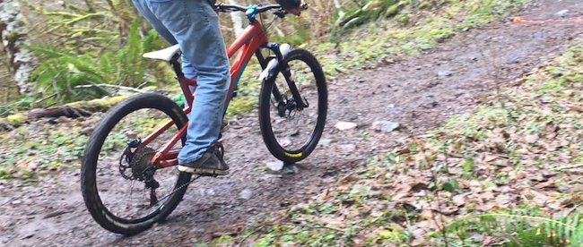
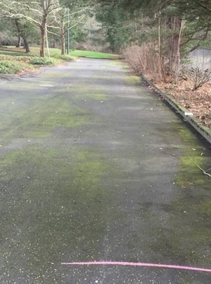
- A bicycle will coast down a fixed distance, in a straight line, from one fixed marker to the next with no pedaling or braking.
- An assistant will record the elapsed time.
- The distance and average slope of the test track will be recorded (probably 100 meters and about 12 degrees). Due to what we learned about gradient resistance from our on-line research, we went with the smallest degrees which allowed the bike to roll. Used 20 meters instead of 100 meters)
- Winds must be 5mph or less as to not impact results.
- Runs will be done with tires at 50PSI, 40PSI, 30PSI, 20PSI, and 10PSI.
- This test will be conducted once on asphalt and once on a rough surface (probably a logging road, preferably with 1-2 inch diameter gravel and some irregularities such as holes and ruts). Ended up using a motorcycle trail with large rocks solidly embedded into the surface. Was worried that gravel would deflect and compress and really be testing a soft surface. Wanted to test a hard surface, but a rough one.


Data Collection
I will be using the programming language R and RStudio which is an IDE (Integrated Development Environment) for R, to analyze, model, and visualize the data I have collected, and Rstudio’s rmarkdown package to communicate my results and answer the questions in the conclusion section.
First, I’ll load the libraries I need in R:
#Load the required libraries for analyis, modeling, and visualization in R
library(tidyverse)
library(broom)
library(modelr)
library(plotly)
library(grid)
library(gridExtra)
Next, I will create data frames for the data I collected for both surfaces in R:
- Smooth surface (asphalt)
- Rough surface (motorcycle trail with large rocks solidly embedded into the surface).
#Create vectors for Air Pressure in PSI, recorded Elapsed time in secs for the bike to travel 20 meters on Smooth and Rough Road
# Tire_Air_Pressure_PSI <- c(50, 50, 50, 40, 40, 40, 30, 30, 30, 20, 20, 20, 10, 10, 10)

Tire_Air_Pressure_PSI <- rep(c(50,40,30,20,10), each =3)
Elapsed_Time_Sec_SmR <- c(9.15, 9.35, 9.42, 9.83, 9.97, 9.77, 10.13, 10.52, 10.27, 11.05, 10.47, 11.09, 12.09, 11.52, 11.15)
Elapsed_Time_Sec_RgR <- c(12.95, 12.10, 13.12, 12.87, 13.44, 13.77, 13.02, 13.62, 13.54, 13.57, 13.80, 14.02, 14.89, 15.02, 15.66)

#bind the Air Pressure, Elapsed time vectors to create a data frame/tibble
Data_for_BikeRuns <- tibble(Tire_Air_Pressure_PSI, Elapsed_Time_Sec_SmR, Elapsed_Time_Sec_RgR)

#View the table of Data_for_BikeRuns
Data_for_BikeRuns
## # A tibble: 15 × 3
## Tire_Air_Pressure_PSI Elapsed_Time_Sec_SmR Elapsed_Time_Sec_RgR
## <dbl> <dbl> <dbl>
## 1 50 9.15 12.95
## 2 50 9.35 12.10
## 3 50 9.42 13.12
## 4 40 9.83 12.87
## 5 40 9.97 13.44
## 6 40 9.77 13.77
## 7 30 10.13 13.02
## 8 30 10.52 13.62
## 9 30 10.27 13.54
## 10 20 11.05 13.57
## 11 20 10.47 13.80
## 12 20 11.09 14.02
## 13 10 12.09 14.89
## 14 10 11.52 15.02
## 15 10 11.15 15.66Next, I will plot and visualize the collected data-set using the ggplot function and plotly.
smooth_title <- c("Smooth Surface")
rough_title <- c("Rough Surface")

own_plot_function <- function(df, manipulated_var, response_var, plottitle) {
  df %>%
    ggplot(aes(x = manipulated_var, y = response_var)) + geom_point(color = "firebrick") + ggtitle(paste("Data for ", plottitle))
}

smooth_surface_plot <- own_plot_function(Data_for_BikeRuns, Tire_Air_Pressure_PSI, Elapsed_Time_Sec_SmR, smooth_title)
rough_surface_plot <- own_plot_function(Data_for_BikeRuns, Tire_Air_Pressure_PSI, Elapsed_Time_Sec_RgR, rough_title)

ggplotly(smooth_surface_plot)
## We recommend that you use the dev version of ggplot2 with `ggplotly()`
## Install it with: `devtools::install_github('hadley/ggplot2')`ggplotly(rough_surface_plot)## We recommend that you use the dev version of ggplot2 with `ggplotly()`
## Install it with: `devtools::install_github('hadley/ggplot2')`Adding the line of best fit to both the data plots. The line of best fit is as close as possible to all points, and as many points above the line as below.
ggplotly(smooth_surface_plot + geom_smooth(method = "lm", se = FALSE, color = "black"))## We recommend that you use the dev version of ggplot2 with `ggplotly()`
## Install it with: `devtools::install_github('hadley/ggplot2')`ggplotly(rough_surface_plot + geom_smooth(method = "lm", se = FALSE, color = "black"))## We recommend that you use the dev version of ggplot2 with `ggplotly()`
## Install it with: `devtools::install_github('hadley/ggplot2')`Observations from Plots as per the topic “Analysis” in our Grade 6 Science Class:
- The plots show a negative correlation; the response variable Elapsed time_sec decreases as the manipulated variable Tire Air Pressure increases, or vice-versa.
- The data points in each plot shows linear relationship.
- The smooth surface data points are closer to the line of best fit than the rough surface data points.
- The difference between the actual observed elapsed time and line of best fit for the smooth surface data is smaller than for the rough surface data. So the residuals for the smooth surface data is smaller than for the rough surface data.
- I expect the \(R^2\) statistic will be higher for the smooth surface versus the rough surface.
- Both these plots tell me that part of my hypothesis which states the rolling resistance of a bicycle tire is inversely related to the air pressure is true.
To prove the other half of my hypothesis, I need to find out the rate of change in the elapsed time in which the bike rolls down the track as the air pressure is decreased by 10 PSI.
To find the rate of change or by how much the elapsed time decreases/increases per 10 PSI increase/decrease, we first need to find the slope of the fitted line or the relationship between the 2 variables by using the simple linear equation \(Y = mx + c\), where m is the slope.
I will first find the slope by writing a function in R, then I will use the linear regression function lm() in R to build a linear model for my dataset.
Our regression line can be written in slope-intercept form:
- Elapsed_Time_in_Secs = (slope)*Tire_Air_Pressure_PSI + (Intercept)
- \(Y = mx + c\)
Transposing, we can calculate the slope manually: \(m = (y_{1}-{y})/(x_{1}-{x})\)
#Create own slope function
own_slope <- function(x, y, x1, y1) {
  m = (y1-y)/(x1-x)
}
So, if I want to calculate the slope between the 2 PSI points 40 PSI and 50 PSI, then we can substitute the x and y values with Elapsed Time and PSI respectively, and make the function call.
slope_40_50_sm <- own_slope(40, 9.83, 50, 9.15)

#Print the slope value for 1 PSI increase
slope_40_50_sm
## [1] -0.068#Since the hypothesis is for 10 PSI
slope_40_50_sm*10## [1] -0.68# To calculate %change in elapsed time, we divide the slope by the elapsed time (y), and multiply it by 100 to change it to percent
Percent_change_Elapsed_Time <- round((slope_40_50_sm*10)/9.83*100, 2)
#Create a single data frame for the slope and % change in elapsed time
single_40_50_data <- tibble(slope_40_50_sm*10, Percent_change_Elapsed_Time)
#print the data frame
single_40_50_data## # A tibble: 1 × 2
## `slope_40_50_sm * 10` Percent_change_Elapsed_Time
## <dbl> <dbl>
## 1 -0.68 -6.92This tells me that for the set of smooth surface data points (40,9.83) and (50,9.15):
- A 10 PSI increase (40 to 50 PSI) causes the elapsed time to decrease by -0.68 and that the % change in Elapsed time in which the bike rolls down the track is -6.92.
- For these two smooth surface data points, my hypothesis is off by -3.92%.
I can manually calculate the slope for each of the 15 observations in each of my datasets, and figure out the % change in the Elapsed time in which our bike rolls down the track, but I will do this with the predicted elapsed time values using the linear modeling function lm().
#The lm() function needs the response variable(Elapsed_Time_Sec_SmR) and the manipulated (Tire_Air_Pressure_PSI) variable, and the data that contains those variables.

model_lm_smooth <- lm(Elapsed_Time_Sec_SmR ~Tire_Air_Pressure_PSI, data = Data_for_BikeRuns)

#To see the summary of the model
summary(model_lm_smooth)
##
## Call:
## lm(formula = Elapsed_Time_Sec_SmR ~ Tire_Air_Pressure_PSI, data = Data_for_BikeRuns)
##
## Residuals:
## Min 1Q Median 3Q Max
## -0.4727 -0.1180 0.0200 0.1383 0.5900
##
## Coefficients:
## Estimate Std. Error t value Pr(>|t|)
## (Intercept) 12.05733 0.15852 76.06 < 2e-16 ***
## Tire_Air_Pressure_PSI -0.05573 0.00478 -11.66 2.95e-08 ***
## ---
## Signif. codes: 0 '***' 0.001 '**' 0.01 '*' 0.05 '.' 0.1 ' ' 1
##
## Residual standard error: 0.2618 on 13 degrees of freedom
## Multiple R-squared: 0.9127, Adjusted R-squared: 0.906
## F-statistic: 136 on 1 and 13 DF, p-value: 2.946e-08While the summary for the model contains all the statistics to explain the result, I will focus only on the ones I understand and taught in our Grade 6 class.
I will use lm() and tidy functions in tidyverse, modelr, and broom libraries in R as shown in Garrett’s Grolemund’s MasterTidyVerse notes. This will provide me with important statistics in a user friendly format:
- An average slope/rate of change of my response variable to the 10 PSI change of my manipulated variable.
- The R-squared statistic (\(R^2\)) which is a number that tells us how well the model fits the actual elapsed data points.
- The Residual statistic which is the difference between my actual Elapsed time data points and the predicted data points.
- The predicted values for my response variable.
#For Smooth test results, use the lm function passing the response and manipulated variables

#Apply lm to the smooth surface data
mod_smooth_1 <- Data_for_BikeRuns %>%
  lm(Elapsed_Time_Sec_SmR ~Tire_Air_Pressure_PSI, data = .)

#Apply lm to the rough surface data
mod_rough <- Data_for_BikeRuns %>%
  lm(Elapsed_Time_Sec_RgR ~Tire_Air_Pressure_PSI, data = .)

#To get the intercept and slope, I'll use the tidy() function from the broom library
smooth_slp_intcpt <- mod_smooth_1 %>%
  tidy() %>%
  select(term, estimate, std.error)

smooth_slp_intcpt
## term estimate std.error
## 1 (Intercept) 12.05733333 0.158523314
## 2 Tire_Air_Pressure_PSI -0.05573333 0.004779658#Do the same for the rough data set
rough_slp_intcpt <- mod_rough %>%
tidy() %>%
select(term, estimate, std.error)
rough_slp_intcpt## term estimate std.error
## 1 (Intercept) 15.30367 0.300061774
## 2 Tire_Air_Pressure_PSI -0.05370 0.009047203Visualization of the model: Used Example from Garrett’s Grolemund’s MasterTidyVerse notes
#Plot the predicted values
Smooth_Data_plot1 <- Data_for_BikeRuns %>%
  add_predictions(mod_smooth_1) %>%
  ggplot(aes(x = Tire_Air_Pressure_PSI)) +
  geom_point(aes(y = Elapsed_Time_Sec_SmR), color = "firebrick") +
  geom_line(aes(y = pred))

#Plot the residuals
Smooth_Data_plot2 <- Data_for_BikeRuns %>%
  add_residuals(mod_smooth_1) %>%
  ggplot(aes(resid)) +
  geom_freqpoly(binwidth = 0.5)


grid.arrange(Smooth_Data_plot1,Smooth_Data_plot2, top = "Smooth Surface Data plots: Predicted, Residuals")
#Plot the residualsFor the smooth surface, the residual plot tells us that the predictions from the observed values are not very far off.
#Plot the predicted values
Rough_Data_plot1 <- Data_for_BikeRuns %>%
  add_predictions(mod_rough) %>%
  ggplot(aes(x = Tire_Air_Pressure_PSI)) +
  geom_point(aes(y = Elapsed_Time_Sec_RgR), color = "firebrick") +
  geom_line(aes(y = pred))

#Plot the residuals
Rough_Data_plot2 <- Data_for_BikeRuns %>%
  add_residuals(mod_rough) %>%
  ggplot(aes(resid)) +
  geom_freqpoly(binwidth = 0.5)

grid.arrange(Rough_Data_plot1,Rough_Data_plot2, top = "Rough Surface Data plots: Predicted, Residuals")
Repeating the same commands and code for both the smooth and rough data points is not very efficient, so I will use the examples of the map() functions from the library purrr and use it with the tidy(), glance() and augment() functions, as provided in Garrett’s Grolemund’s MasterTidyVerse notes from RStudio conference 2017.
#First I will create the formulas with the Elapsed time and PSI variables so we can map it to lm()

formulas_for_lm <- list(
  mod_smooth <- Elapsed_Time_Sec_SmR ~Tire_Air_Pressure_PSI,
  mod_rough <- Elapsed_Time_Sec_RgR~Tire_Air_Pressure_PSI
)

#'ll map the formulas created to function lm, and provide it the Data_for_BikeRuns data set to get the intercept and slope values using tidy for both the smooth and rough data sets

slope_intercept <- formulas_for_lm %>%
  map(lm, data = Data_for_BikeRuns) %>%
 map_df(tidy, .id = "model") %>%
  select(model, term, estimate, std.error)

slope_intercept
## model term estimate std.error
## 1 1 (Intercept) 12.05733333 0.158523314
## 2 1 Tire_Air_Pressure_PSI -0.05573333 0.004779658
## 3 2 (Intercept) 15.30366667 0.300061774
## 4 2 Tire_Air_Pressure_PSI -0.05370000 0.009047203For the smooth surface data points (model 1), the statistics from the model shows that:
- For every 1 PSI increase in the pressure of the tire, the required time (elapsed time) to complete the travel distance goes down by -0.0557333 secs.
- Therefore, a 10 PSI increase causes the elapsed time to decrease by -0.5573333 secs. Or conversely, for 10 PSI decrease, the required time to complete the travel distance goes up by -0.5573333 secs.
- The intercept tells me that at 0 PSI, the elapsed time for the bike to roll down the 20 meters track is 12.0573333 secs; this is not possible because a tire with 0 PSI will not be able to roll.
- The std.error shows that the time required by the bike to complete the 20 meters travel distance can vary by 0.0047797 secs.
Similarly for the rough surface data points(model 2):
- For every 1 PSI increase in the pressure of the tire, the required time (elapsed time) to complete the travel distance goes down by -0.0537 secs.
- Therefore, a 10 PSI increase causes the elapsed time to decrease by -0.537 secs. Or conversely, for 10 PSI decrease, the required time to complete the travel distance goes up by -0.537 secs.
- The intercept tells me that at 0 PSI, the elapsed time for the bike to roll down the 20 meters track is 15.3036667 secs; this is not possible because a tire with 0 PSI will not be able to roll.
- The std.error shows that the time required by the bike to complete the 20 meters travel distance can vary by 0.0090472 secs.
Now, let’s extract the \(R^2\) for each of the models.
#I'll map the formulas created to function lm(), and provide it the Data_for_BikeRuns data set, and use glance() to get the r-squared values
Rsquared_fit <- formulas_for_lm %>%
  map(lm, data = Data_for_BikeRuns) %>%
  map_df(glance, .id = "model") %>%
  select(model, r.squared, p.value)
#Print the R-Squared values
Rsquared_fit
## model r.squared p.value
## 1 1 0.9127329 2.946122e-08
## 2 2 0.7304615 4.939636e-05For the smooth surface data set, the \(R^2\) value of 0.9127329 is close to 1 which tells me the fit of the model is really good. It is a high R.squared fit for the smooth data set and an Okay fit on the rough data set whose \(R^2\) value is 0.7304615. This tells me that if I were choose tire pressure(measured in PSI) as an important measurement that could help explain how the rolling resistance of the bike would vary based on tire pressure(PSI), then I would be correct. It is why we get a high R.squared fit.
Finally to get the predicted Elapsed time values (the line of best fit values) and how off the predicted values are compared to our actual elapsed time data, I will use the augment() function.
#To get the predictions and residuals from the model along with the original data points, I will use the augment() function

predicted_residual_val <- formulas_for_lm %>%
  map(lm, data = Data_for_BikeRuns) %>%
  map_df(augment, .id = "model") %>%
  select(model, Elapsed_Time_Sec_SmR, Tire_Air_Pressure_PSI, .fitted, .resid, Elapsed_Time_Sec_RgR)

predicted_residual_val
## model Elapsed_Time_Sec_SmR Tire_Air_Pressure_PSI .fitted .resid
## 1 1 9.15 50 9.270667 -0.12066667
## 2 1 9.35 50 9.270667 0.07933333
## 3 1 9.42 50 9.270667 0.14933333
## 4 1 9.83 40 9.828000 0.00200000
## 5 1 9.97 40 9.828000 0.14200000
## 6 1 9.77 40 9.828000 -0.05800000
## 7 1 10.13 30 10.385333 -0.25533333
## 8 1 10.52 30 10.385333 0.13466667
## 9 1 10.27 30 10.385333 -0.11533333
## 10 1 11.05 20 10.942667 0.10733333
## 11 1 10.47 20 10.942667 -0.47266667
## 12 1 11.09 20 10.942667 0.14733333
## 13 1 12.09 10 11.500000 0.59000000
## 14 1 11.52 10 11.500000 0.02000000
## 15 1 11.15 10 11.500000 -0.35000000
## 16 2 NA 50 12.618667 0.33133333
## 17 2 NA 50 12.618667 -0.51866667
## 18 2 NA 50 12.618667 0.50133333
## 19 2 NA 40 13.155667 -0.28566667
## 20 2 NA 40 13.155667 0.28433333
## 21 2 NA 40 13.155667 0.61433333
## 22 2 NA 30 13.692667 -0.67266667
## 23 2 NA 30 13.692667 -0.07266667
## 24 2 NA 30 13.692667 -0.15266667
## 25 2 NA 20 14.229667 -0.65966667
## 26 2 NA 20 14.229667 -0.42966667
## 27 2 NA 20 14.229667 -0.20966667
## 28 2 NA 10 14.766667 0.12333333
## 29 2 NA 10 14.766667 0.25333333
## 30 2 NA 10 14.766667 0.89333333
## Elapsed_Time_Sec_RgR
## 1 NA
## 2 NA
## 3 NA
## 4 NA
## 5 NA
## 6 NA
## 7 NA
## 8 NA
## 9 NA
## 10 NA
## 11 NA
## 12 NA
## 13 NA
## 14 NA
## 15 NA
## 16 12.95
## 17 12.10
## 18 13.12
## 19 12.87
## 20 13.44
## 21 13.77
## 22 13.02
## 23 13.62
## 24 13.54
## 25 13.57
## 26 13.80
## 27 14.02
## 28 14.89
## 29 15.02
## 30 15.66To calculate the percentage change on the Elapsed time when the PSI is changed by 10 PSI (second part of my hypothesis), I will use the slope and divide it by the predicted Elapsed Time values from the model.
perc_chg_smooth <- predicted_residual_val%>%
  filter(model ==1) %>%
  distinct(Tire_Air_Pressure_PSI,.fitted) %>%
  mutate(perc_chg = ((slope_intercept$estimate[[2]]*10)/lead(.fitted,1))*100, Delta_myHypothesis = (perc_chg-(-3)))

perc_chg_rough <- predicted_residual_val%>%
  filter(model ==2) %>%
  distinct(Tire_Air_Pressure_PSI,.fitted) %>%
  mutate(perc_chg = ((slope_intercept$estimate[[4]]*10)/lead(.fitted,1))*100, Delta_myHypothesis = (perc_chg-(-3)))

perc_chg_smooth
## Tire_Air_Pressure_PSI .fitted perc_chg Delta_myHypothesis
## 1 50 9.270667 -5.670872 -2.670872
## 2 40 9.828000 -5.366543 -2.366543
## 3 30 10.385333 -5.093213 -2.093213
## 4 20 10.942667 -4.846377 -1.846377
## 5 10 11.500000 NA NAFor the smooth surface data set, it appears that my hypothesis of an increase of 3% in elapsed time for every 10 PSI decrease is not very accurate to the average percent change of -5.2442512 of the predicted values.
perc_chg_rough## Tire_Air_Pressure_PSI .fitted perc_chg Delta_myHypothesis
## 1 50 12.61867 -4.081891 -1.0818912
## 2 40 13.15567 -3.921807 -0.9218073
## 3 30 13.69267 -3.773806 -0.7738059
## 4 20 14.22967 -3.636569 -0.6365688
## 5 10 14.76667 NA NAFor the rough surface data set, it appears that my hypothesis of an increase of 3% in elapsed time for every 10 PSI decrease is very close to the average percent change of -3.8535183 of the predicted values.
Extra
Interpolation: Interpolation is where we find a value inside our set of data points. Interpolating to get an estimate of the elapsed time when PSI is 15
Elapsed_15PSI <- mod_smooth_1$coefficients[[2]]*15 + mod_smooth_1$coefficients[[1]]

Elapsed_15PSI
## [1] 11.22133Extrapolation: Extrapolation is where we find a value outside our set of data points Extrapolating to get an estimate of the elapsed time when PSI is 60
Elapsed_60PSI <- mod_smooth_1$coefficients[[2]]*60 + mod_smooth_1$coefficients[[1]]

Elapsed_60PSI
Conclusion
The Tire Air Pressure PSI affects the rolling resistance of a Mountain Bike (measured in elapsed time secs), as we have proved that it is negatively correlated, the slope or rate of change per 10 PSI is -0.5573333 (for smooth surface) and -0.537 secs(for rough surface) which means the air pressure and rolling resistance are inversely related.
The correct part of my hypothesis is that for every 10 PSI decrease, the elapsed time in which the bike rolls down the track will increase. The incorrect part is the % of decrease which is an average of -5.2442512 for the smooth surface, and an average of -3.8535183 for the rough surface, versus the 3% in my hypothesis.
The problems I encountered when doing the test are as follows:
- Started raining when we tested the rolling resistance on the rough surface
- Hard to get the right terrain and incline for our test. As it is a wet winter it took a couple hours to find a spot for the rough test. We wanted a surface that was rough but not soft so we needed a test track with a minimum of soil and vegetation.
- Had to use a slightly steeper 4 degree grade for the rough surface test as the bike would not remain stable using the 3 degree grade of the smooth surface test.
- Difficult to start moving consistently for each test.
The additional piece I’d like to investigate:
- Soft versus hard surface. If the trail is soft mud, or contains a lot of soft vegetation, does tire PSI affect the rolling resistance?
Our test proves that:
- Higher air pressure does roll faster. This matters because mountain bikes are limited to the power provided by a human, so efficiency is a top priority.
- Traction is also very important, and lower pressure provides better traction.
- This test makes it easier to make a data-driven decision when a bike rider has to make the trade-off between traction and efficiency.
Background Information
-They claim tires inflated to a high PSI are faster on a smooth surface and tires inflated to a low PSI are faster on a rough surface. This is a biased source and they offer no evidence of their claims. Definitions from this source: - Rolling resistance: Energy that is lost when the tire is rolling - Air resistance : Resistance to air that rises in a squared ratio with increased speed. - Gradient resistance : The main resistance to overcome when riding uphill (Due to gradient resistance we modified our test to use the smallest grade possible instead of what we originally proposed).
Various road bicycle tires were tested against a smooth, steel drum. The graph shows a rolling resistance decreasing with increased air pressure. The source concludes that the returns from increasing pressure diminished at a certain point. Note that these tires are quite smoother and smaller than mountain bike tires.
Has mathematical formulas which show more air pressure resulting in less rolling resistance. Note Math is outside of grade level.
R Challenges
- I did not understand what data_grid() from the modelr library does
- Could not replace Model 1, 2 with names (smooth and rough) that would identify the model
- Could not show my plots side by side using ggplot and plotly.
- Difficult to remember which functions (tidy, glance, augment) extracted which pieces of the lm model statistics.
Overall, the project was long but fun, and I look forward to next year’s STEM Expo. I’m also hoping to build a basic shiny app to demo my expo results.
I’d like to thank RStudio (Garrett Grolemund, J.J. Allaire, Hadley Wickham, Roger Oberg, ) and DataCamp (Nick Carchedi, Jonathan Cornelissen) for their kindness and all the help and encouragement they have given me to learn R. Thank you so much.
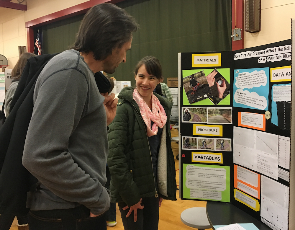
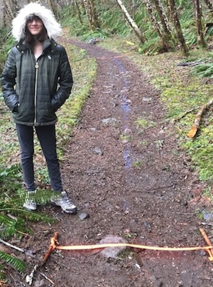
STEM Expo Pictures