Learning Bivariate realtionship in my math class
library(tidyverse)## ── Attaching packages ─────────────────────────────── tidyverse 1.2.1 ──## ✔ ggplot2 3.1.0 ✔ purrr 0.3.0
## ✔ tibble 2.0.1 ✔ dplyr 0.7.8
## ✔ tidyr 0.8.2 ✔ stringr 1.3.1
## ✔ readr 1.3.1 ✔ forcats 0.3.0## ── Conflicts ────────────────────────────────── tidyverse_conflicts() ──
## ✖ dplyr::filter() masks stats::filter()
## ✖ dplyr::lag() masks stats::lag()fertilizer <- c(5, 10, 15, 20, 25, 30)
height_of_plant <- c(14, 17, 21, 31, 33, 40)
plant_data <- tibble(fertilizer, height_of_plant)
ggplot(plant_data, aes(x = fertilizer, y = height_of_plant)) + geom_point() + geom_smooth(method = lm)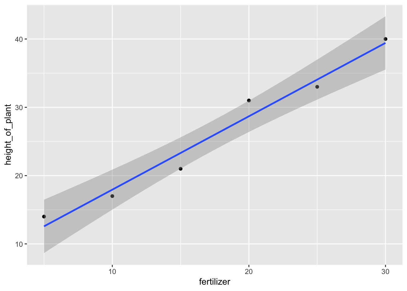
y = mx + c
m = (y2 - y1)/(x2 - x1)
m = (17-14)/(10-5)
plant_data
m
A_data <- tibble(weekend = c("feb6", "feb13", "feb20", "feb27", "march6", "march13"), time_min = c(68, 88, 35, 150, 104, 80), distance_miles = c(7, 17, 3.5, 25, 14, 11))
A_data %>% ggplot(aes(x = distance_miles, y = time_min)) + geom_point() + geom_smooth(method = lm)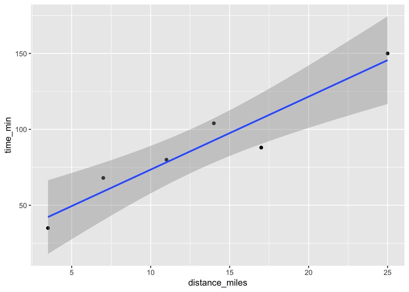
A_data## # A tibble: 6 x 3
## weekend time_min distance_miles
## <chr> <dbl> <dbl>
## 1 feb6 68 7
## 2 feb13 88 17
## 3 feb20 35 3.5
## 4 feb27 150 25
## 5 march6 104 14
## 6 march13 80 11my_slope <- function(y2, y1, x2, x1) {
m = (y2-y1)/(x2-x1)
return(m)
}
my_slope(35, 88, 3.5, 17)## [1] 3.925926my_slope(133,127, 169,166.4)## [1] 2.307692my_intercept <- function(y, x, m) {
c= y-m*x
return(c)
}
2.30*228.6 - 272.7## [1] 253.08my_intercept(139, 179, 2.30)## [1] -272.7newtons_revenge <- tibble(Height = c(166.4,169,172.8,179,170,183,162.5,165,157.5,165,169,156), reach = c(127,133,133,139,139,137,121,126,128,123,132,119))
newtons_revenge## # A tibble: 12 x 2
## Height reach
## <dbl> <dbl>
## 1 166. 127
## 2 169 133
## 3 173. 133
## 4 179 139
## 5 170 139
## 6 183 137
## 7 162. 121
## 8 165 126
## 9 158. 128
## 10 165 123
## 11 169 132
## 12 156 119ggplot(newtons_revenge, aes(x = Height, y = reach)) + geom_point() + geom_smooth(method = lm)
str(newtons_revenge)## Classes 'tbl_df', 'tbl' and 'data.frame': 12 obs. of 2 variables:
## $ Height: num 166 169 173 179 170 ...
## $ reach : num 127 133 133 139 139 137 121 126 128 123 ...newtons_revenge_1 <- newtons_revenge %>% mutate(heightchange = Height-lag(Height), reachchange = reach-lag(reach), slope = reachchange/heightchange)
str(newtons_revenge_1)## Classes 'tbl_df', 'tbl' and 'data.frame': 12 obs. of 5 variables:
## $ Height : num 166 169 173 179 170 ...
## $ reach : num 127 133 133 139 139 137 121 126 128 123 ...
## $ heightchange: num NA 2.6 3.8 6.2 -9 ...
## $ reachchange : num NA 6 0 6 0 -2 -16 5 2 -5 ...
## $ slope : num NA 2.308 0 0.968 0 ...newtons_revenge_1## # A tibble: 12 x 5
## Height reach heightchange reachchange slope
## <dbl> <dbl> <dbl> <dbl> <dbl>
## 1 166. 127 NA NA NA
## 2 169 133 2.60 6 2.31
## 3 173. 133 3.8 0 0
## 4 179 139 6.20 6 0.968
## 5 170 139 -9 0 0
## 6 183 137 13 -2 -0.154
## 7 162. 121 -20.5 -16 0.780
## 8 165 126 2.5 5 2
## 9 158. 128 -7.5 2 -0.267
## 10 165 123 7.5 -5 -0.667
## 11 169 132 4 9 2.25
## 12 156 119 -13 -13 1newtons_revenge_1 <- newtons_revenge %>% mutate(heightchange = Height-lag(Height), reachchange = reach - lag(reach), slope = reachchange/heightchange)
newtons_revenge_1## # A tibble: 12 x 5
## Height reach heightchange reachchange slope
## <dbl> <dbl> <dbl> <dbl> <dbl>
## 1 166. 127 NA NA NA
## 2 169 133 2.60 6 2.31
## 3 173. 133 3.8 0 0
## 4 179 139 6.20 6 0.968
## 5 170 139 -9 0 0
## 6 183 137 13 -2 -0.154
## 7 162. 121 -20.5 -16 0.780
## 8 165 126 2.5 5 2
## 9 158. 128 -7.5 2 -0.267
## 10 165 123 7.5 -5 -0.667
## 11 169 132 4 9 2.25
## 12 156 119 -13 -13 1my_intercept(127, 166.4, 2.3)## [1] -255.72my_intercept(127, 166.4, 0.96)## [1] -32.744my_intercept(133,169, 0)## [1] 133ggplot(newtons_revenge, aes(x = Height, y = reach))+geom_point()+geom_smooth(method = lm)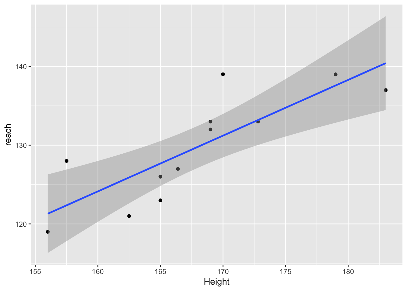
model_lm_smooth <- lm(reach ~Height, data = newtons_revenge)
summary(model_lm_smooth)
##
## Call:
## lm(formula = reach ~ Height, data = newtons_revenge)
##
## Residuals:
## Min 1Q Median 3Q Max
## -4.9030 -2.5800 -0.9301 1.7448 7.7867
##
## Coefficients:
## Estimate Std. Error t value Pr(>|t|)
## (Intercept) 10.8465 26.6820 0.407 0.69293
## Height 0.7080 0.1587 4.461 0.00121 **
## ---
## Signif. codes: 0 '***' 0.001 '**' 0.01 '*' 0.05 '.' 0.1 ' ' 1
##
## Residual standard error: 4.139 on 10 degrees of freedom
## Multiple R-squared: 0.6655, Adjusted R-squared: 0.6321
## F-statistic: 19.9 on 1 and 10 DF, p-value: 0.001215