Grade 5: Our Journey Through R

Description

Started: December 27th, 2015

Updated: January 27, 2016

Project: Explore and Calculate Statistical Concepts (mean, median, and range) we learned during our Grade 5 Math class, in a programming language “R”.

Deliverables:

1. A Website that details our project’s reproducible research (Started: Dec 27th, 2015 - Done: February 6th, 2016)
2. Our mean, median, and range functions written in R (Started: Mid-December 2015 - Done: January 22nd, 2016)
3. Plots of our data using the ggvis package (Done: January 29th, 2016)
4. A web Application (shiny app) in R (Work In Progress)
5. Certification of Completion of Introduction to R by Datacamp (Done: January 7th, 2016)

Our Journey:

1. We started our project on October 1st, 2015.

2. We started learning the R programming language by signing up for an interactive Introduction to R course offered by DataCamp. The course has 6 chapters: Intro to Basics, Vectors, Matrices, Factors, Data Frames, Lists.

3. We will be completing all the 6 chapters and programming exercises by the end of next week, January 7th, 2016. This is Done

4. We started our website for our project’s reproducible research on December 27th, 2015. Updated it on January 25th/27th 2016 and February 6th/8th 2016

5. We have completed building our R application, but we will attempt to build the R Shiny web application by the first week of February 2016.

Below is a sample of R code that we have written so far:

#Build the character and numeric vectors and assign it to the variables
districts<-c("District1", "District2", "District3", "District4", "District5", "District6", "District7", "District8")
months<- c ("May", "June", "July", "Aug", "Sep", "Oct", "Nov", "Dec")
score<- c (5,7,15,12,0,2,6,6)

#Build the data frame NaughtyNice using the data.frame function
NaughtyNice <-data.frame(districts, months, score)

#Print the dataframe NaughtyNice
NaughtyNice

##   districts months score
## 1 District1    May     5
## 2 District2   June     7
## 3 District3   July    15
## 4 District4    Aug    12
## 5 District5    Sep     0
## 6 District6    Oct     2
## 7 District7    Nov     6
## 8 District8    Dec     6

#plot the score vector on the y-axis and districts on the x-axis
plot(NaughtyNice$score, type = "p", xlab = "Districts", ylab = "Scores")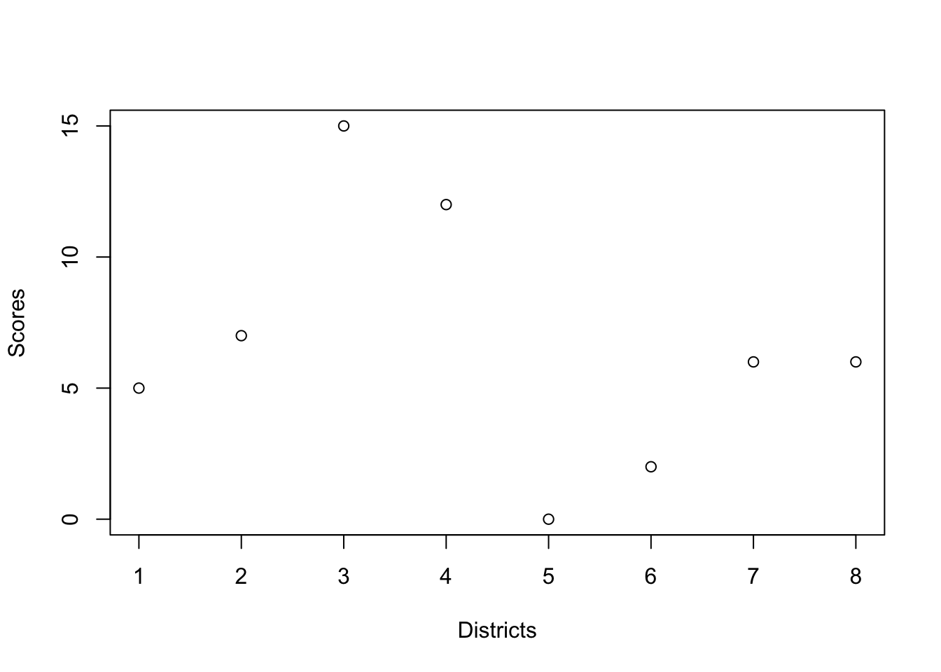

#plot(NaughtyNice)

#load required libraries
library(ggvis)
library(dplyr)
library(gtools)

Using the read.csv function and ggvis package for plots

#we can also read data files in R by using the function read; in this case we are reading a csv file that contains data for our naughtynice score and store it in a dataframe object csvnicenaughty
csvnicenaughty<- read.csv("../../static/data/testscore.csv", stringsAsFactors = F)

#Then we plot the score from the data file using the ggvis plotting package in R
#We use the %>% or pipe function which passes saved data to the function group_by
#which then passes it to the function ggvis for the plot.  The %>% lets makes the 
#code easier to write and understand. 

csvnicenaughty %>% group_by(Districts) %>% ggvis(x = ~Districts, y = ~Score) %>% layer_bars(fill = ~Districts)

#We can also use the box-plot or the box-whisker plot using the ggvis package, so we can see the median and range of the scores.
csvnicenaughty %>% group_by(Districts) %>% ggvis(x = ~Districts, y = ~Score) %>% layer_boxplots(fill = ~Districts)

#We will now write our own functions and compare the result to the same in-built functions in R

#Our mean function
ownmean <- function(x) {
  meanresult <- sum(x)/length(x)
  return(meanresult)
}

#Call own mean function on csvnicenaughty data
ownmean(csvnicenaughty$Score)

## [1] 6.5625

#Compare to built-in mean function in R
mean(csvnicenaughty$Score)

## [1] 6.5625

#Our range function
ownrange <- function(x) {
  totalnum <- length(x)
  sortednnice <- sort(x, decreasing = FALSE)
  rangeresult <- sortednnice[totalnum]-sortednnice[1]
  return(rangeresult)
}

#Call own range function on csvnicenaughty data
ownrange(csvnicenaughty$Score)

## [1] 14

#Compare to built-in range function in R
range(csvnicenaughty$Score)

## [1]  0 14

ownmedian <- function(x) {
  sortednnice <- sort(x, decreasing = FALSE)
  #divide the total number of scores by 2 to find the mid point
  halflength <- length(x)/2
    if (odd(length(x))) {
      sortednnice[halflength+1]
    }
  else {
     (sortednnice[halflength]+sortednnice[halflength+1])/2
  }
  
}

#Call our own median function on our stored data
ownmedian(csvnicenaughty$Score)

## [1] 6

#call R's in-built median function
median(csvnicenaughty$Score)

## [1] 6

Challenges we faced

These were the challenges that we had to deal with when learning R and completing the project:

1. Learning the new syntax of R
2. Writing the functions
3. Finding the mistakes in our R code

The Fun Part

1. Seeing our code work
2. Collecting the data points
3. Creating the dataframe

Future with R

We plan to continue learning R by:

1. Completing Intermediate courses offered by DataCamp
2. Making a shiny application
3. Learning the ggvis package offered by DataCamp

Pictures of the Science Fair